The Multiple Layer Search tab houses the most comprehensive search in ELAN. Similar to the Single Layer Search tab a Query History is kept, enabling the user to go back and forward a query by clicking the and respectively. It it also possible to either save or load a previously saved query. To do so, click either the or the button. Queries are saved in XML format.
The two modes / and // are also similar to the second tab. The first new element is the -button. Clicking this button will clear all data of a query.
A new option has been included into the menu containing all the different types of matches (i.e. substring match, exact match, regular expression): variable match. As the name says, it has to do with using variables, and it can be used every time you want to search for two or more annotations, contained in two or more different tiers, reporting the same text and/or the same time alignment. See the image below for an example:
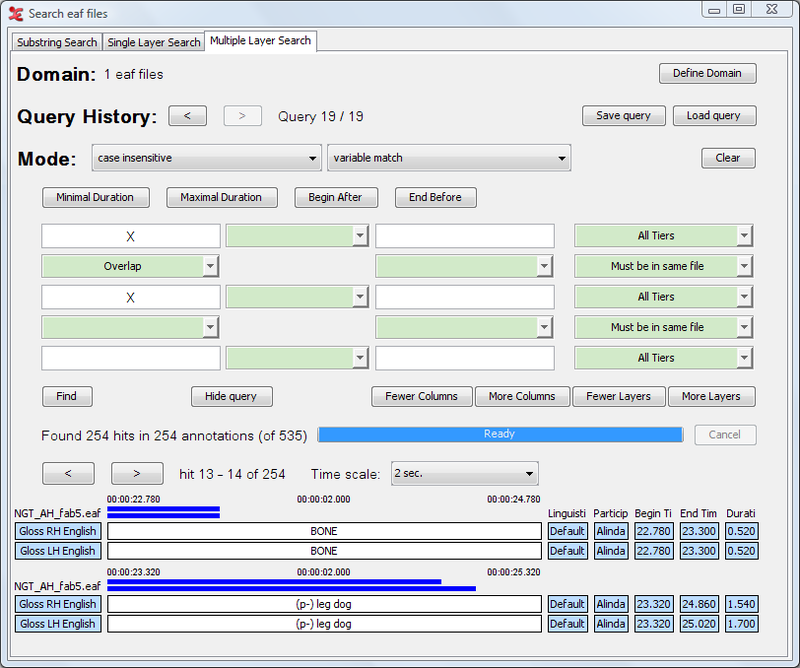
As you can see in the example, the variable 'X' can match any same value of annotations that meet all other constraints. They are in the same time-frame (overlap) and reside in the same file (the base constraint is ) . In this case 'BONE' is found in the tier 'Gloss RH English' and in 'Gloss LH English', the same for the value '(p-) leg dog'.
It is possible to use more than one variable, e.g. X and Y. This is especially useful in those cases where more than two query fields are filled in.
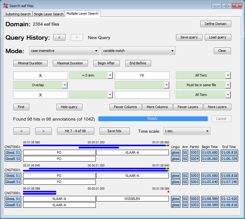
X and Y can either match different values or the same value. If a variable should be unique, i.e. should never match the same value as any of the other variables, it should be preceded by an exclamation mark, e.g. !Y.
The buttons and enables you to constrict the minimal and maximal duration of each result. When you click on one of the buttons, a dialog window appears, e.g.:
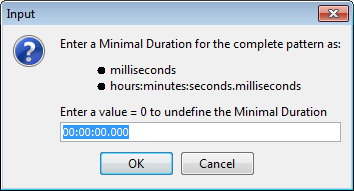
Here you can enter the minimal or maximal duration as the total number of
milliseconds or in hours:minutes:seconds.milliseconds. A value of 0 milliseconds or
00:00:00.000 yields as undefined. Searching for annotations with a maximum duration
being less then the minimum duration is impossible. Hence, entering conflicting values
results in an error message saying that the combination is impossible. After entering a
correct duration, it will be displayed in the corresponding button.
The buttons and give a dialog similar to that of the previous two buttons. They give the possibility to restrict the annotations in the result to begin after a certain time and end before a certain time. Entering a Begin After-time that is greater than the End Before-time or vice versa results in an error message saying it is impossible. After entering a correct time, it will be displayed in the corresponding button.
Search string and constraints
Beneath the buttons discussed above, you will find a table consisting of white and green fields. Search strings are entered in the white fields while a green field between two non-empty white fields must contain a constraint. The fields on one row give the search strings and constraints to be matched by annotations on one tier. The result of having two or more rows in the query table is that the search engine may find annotations on two or more tiers as one hit. Furthermore, it is possible to restrict the search to one (type of) tier for each row by choosing the appropriate option in the pull-down menu on the right of each row.
Let us first take a look at search strings and constraints in one row. If you enter two search strings in two white fields separated by a green field, you must fill in that green field i.e. make a constraint. Clicking the arrow on the green field gives a menu offering the following constraints:
: between the annotations containing the two search strings, there must be exactly N annotations.
: between the annotations containing the two search strings, there must be more than N annotations.
: between the annotations containing the two search strings, there must be less than N annotations.
: between the annotations containing the two search strings, there must be exactly X milliseconds.
: between the annotations containing the two search strings, there must be more than X milliseconds.
: between the annotations containing the two search strings, there must be less than X milliseconds.
: there are no constraints.
: clear the current constraint.
When you click on and there is an empty constraint between two non-empty search string fields, you will get an error message. You will also get an error message if there is an empty search string field and constraint fields between two non-empty search string fields.
As we saw earlier the search mechanism on this tab has the possibility to construct a query for two or more tiers (up to eight). Besides the constraints on annotations on a tier, one can also apply constraints on annotations on different tiers. This means that if the search engine has found an annotation that matches a search string on one tier, the engine looks if the search string for another tier can be matched on another tier while considering the constraint that is between the two search strings.
The top down hierarchy of the rows in the query table does not reflect the hierarchy of the tiers in your data. That means, for instance, that search strings and constraints in the upper query table row may be matched by a child tier of the tier that matches search strings and constraints in the middle query table row.
Clicking the arrow in the green field between two search strings gives a menu with the following constraints:
: the begin time and end time of both annotations are the same:

: part of both annotations overlap. This includes the other options Fully aligned, Left overlap, Right overlap, Surrounding and Within.
: the begin time and end time of the annotation matching the lower search string lie before the begin time and end time of the annotation matching the upper search string:

: the begin time and end time of the annotation matching the lower search string lie after the begin time and end time of the annotation matching the upper search string:

: the begin time of the annotation matching the lower search string lies before the begintime of the annotation matching the upper search string and end time of the annotation matching the lower search string lies after the end time of the annotation matching the upper search string:

: the begin time of the annotation matching the lower search string lies after the begintime of the annotation matching the upper search string and end time of the annotation matching the lower search string lies before the end time of the annotation matching the upper search string:

: the begin time of the annotation matching a search string lies after the end time of the annotation matching the other search string:
 or
or 
: a special case that retrieves annotations matching the upper search string that have no (overlapping) annotation on the lower tier. It is not possible to enter a lower search string; contrary to the constraint, which still looks for annotations on the lower tier (namely those that don't overlap), this constraint really looks for no annotation in the timespan of the upper annotation (empty slots). The user interface allows specifying constraints on lower levels and to the left and right of this constraint, but the behavior in that case is undefined!
: the begin time of the annotations matching the upper search string must lie exactly X milliseconds before the begin time of the annotation matching the lower search string.
: the begin time of the annotations matching the upper search string must lie less than X milliseconds before the begin time of the annotation matching the lower search string.
: the begin time of the annotations matching the upper search string must lie more than X milliseconds before the begin time of the annotation matching the lower search string.
: the end time of the annotations matching the upper search string must lie exactly X milliseconds before the begin time of the annotation matching the lower search string.
: the end time of the annotations matching the upper search string must lie less than X milliseconds before the begin time of the annotation matching the lower search string.
: the end time of the annotations matching the upper search string must lie more than X milliseconds before the begin time of the annotation matching the lower search string.
: the begin time of the annotations matching the upper search string must lie exactly X milliseconds before the end time of the annotation matching the lower search string.
: the begin time of the annotations matching the upper search string must lie less than X milliseconds before the end time of the annotation matching the lower search string.
: the begin time of the annotations matching the upper search string must lie more than X milliseconds before the end time of the annotation matching the lower search string.
: the end time of the annotations matching the upper search string must lie exactly X milliseconds before the end time of the annotation matching the lower search string.
: the end time of the annotations matching the upper search string must lie less than X milliseconds before the end time of the annotation matching the lower search string.
: the end time of the annotations matching the upper search string must lie more than X milliseconds before the end time of the annotation matching the lower search string.
: there are no constraints.
: clear the current constraint.
An example of a Multiple Layer Search with constraints is shown below:
As you can see the tiers in the result are indicated by #1 and #2, corresponding to the first and second query table row respectively. The annotations in a tier are surrounded by vertical bars indicating their start and end.
It is possible to add or remove columns and/or layers to your search query. To do so, click the respective button:
It is also possible to hide the query once there are search results. This allows you to see more query results within a single window. This can be helpful when using the Alignment View Section 4.4.3.1.
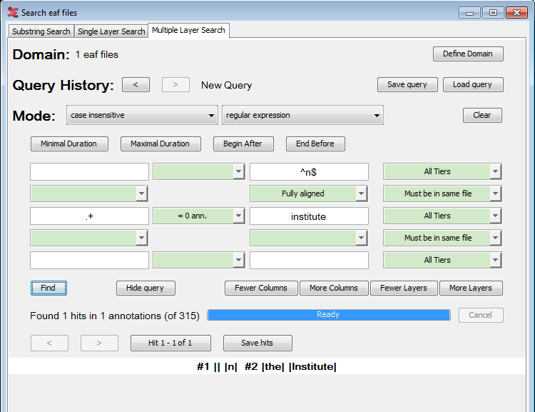
Figure 4.26 also illustrates what to do if you
would like to use both and in one query: use the . In places where you would like to have an exact match use
the ^ and $ signs to match the beginning
and end of a string (e.g. ^of$) otherwise just enter a word for
the substring match.
The figure also show how to use a wildcard to match anything. Instead of using the
# as in the Single Layer Search, you can use the regular
expression .+ to indicate any character (the dot) one or more
times (the plus). See also Appendix A for more on regular
expressions. The NOT(...) construction on the other hand can be used in the Multiple
Layer Search in the same way as describe in Section 4.4.2.
One final but not less important remark concerns the placing of more and less
restrictive search strings. Figure 4.26 shows a very
restrictive search string in the upper row: ^n$. The less
restrictive, or should we say non-restrictive, search string .+ is in the middle row. As
we saw earlier, the hierarchy of the rows in the query does not reflect the hierarchy in
the data. That means that the search string ^n$ could also be
placed in the lower row and not affect the outcome of the search. While this is
perfectly true, we advise you to place restrictive search strings in the left most field
on the upper most row possible and the least restrictive search string in the right most
field of the lowest row possible. The reason for this is the order in which the search
engine considers the search strings in the query. If it finds a restrictive search
string it can filter out all the other possibilities, but if it finds a less restrictive
search string it has to consider all the matches of this search string. In the example
of Figure 4.26 it is clear that if
^n$ is in the bottom row, the search engine first considers all
annotations matching .+ which is in fact all
annotations in the search domain. Because of this, the search takes much more time than
if ^n$ was in the upper row.
From the context-menu (right-click the search results), you van view query results from the Multiple Layer Search in Alignment View:
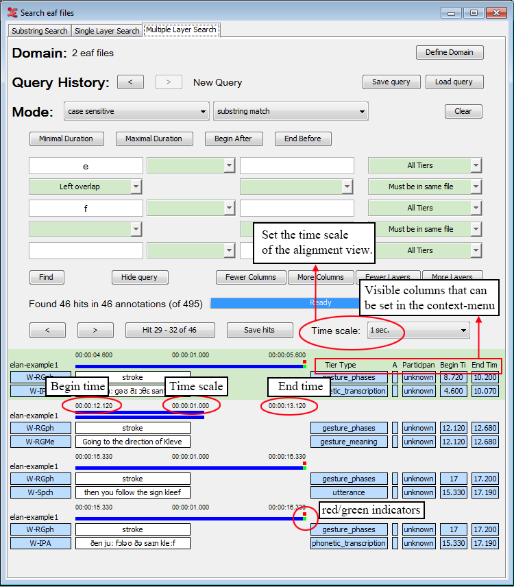
There are a number of options you can set when viewing the query results. Firstly, you can adjust the time scale of the results:
1 sec / 2sec / 5sec / 10 sec / 15 sec / 20 sec / User defined / Scale to fit.
When choosing 'Scale to fit', every query result will be scaled to fit the window, which means the time scale for every result will differ.
There is also the possibility to hide the alignment time scale altogether. To do so, go to the context-menu (right-click) and uncheck by clicking on it.
You can set the visible columns to the right of the query results through the context-menu (right-click anywhere in the results). You can show or hide the following columns:
Tier Type
Annotator
Participant
Begin Time
End Time
Duration
The blue bars above every query result graphically show the duration of each annotation and the position of the annotations with respect to each other.
There are also two indicators visible, depending on the length of the query result and the setting of the time scale. These indicators are either red or green.
A green indicator means that the annotation does not fit in the current time scale. In the example above, the bottom annotation 'and then you see um a man in maybe his fifties' has a duration of 5.060 seconds. The time scale is set to 1 second, so 4.060 seconds are outside the current view.
The red indicator means that the annotation in the query result starts outside of the current time scale. The top annotation 'fifties' overlaps the bottom annotation, but starts at 9.177 seconds. This causes it not to be visible in the current time scale, which is set to display 1 second. You would need to set the time scale to 10 seconds to see both annotations visualised completely (as the blue bars) and how they overlap.